Question:- 2(a) Explain the operation of two-tier client/server architecture. How three-tire client/server architecture is different from it.
Answer:-Understanding DBMS Architecture
A Database Management system is not always directly available for users and applications to access and store data in it. A Database Management system can be centralised(all the data stored at one location), decentralised(multiple copies of database at different locations) or hierarchical, depending upon its architecture.
1-tier DBMS architecture also exist, this is when the database is directly available to the user for using it to store data. Generally such a setup is used for local application development, where programmers communicate directly with the database for quick response.
Database Architecture is logically of two types:
- 2-tier DBMS architecture
- 3-tier DBMS architecture
2-tier DBMS Architecture
2-tier DBMS architecture includes an Application layer between the user and the DBMS, which is responsible to communicate the user’s request to the database management system and then send the response from the DBMS to the user.
An application interface known as ODBC(Open Database Connectivity) provides an API that allow client side program to call the DBMS. Most DBMS vendors provide ODBC drivers for their DBMS.
The two-tier is based on Client Server architecture. The two-tier architecture is like client server application. The direct communication takes place between client and server. There is no intermediate between client and server. Because of tight coupling a 2 tiered application will run faster.
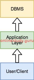
The above figure shows the architecture of two-tier. Here the direct communication happens between client and server, there is no intermediate layer between client and server. The Two-tier architecture is divided into two parts:
- Client Application (Client Tier)
- Database (Data Tier)
On client application side the code is written for saving the data in database server. Client sends the request to server and it process the request & send back with data. The main problem of two tier architecture is the server cannot respond multiple request same time, as a result it cause a data integrity issue. When the developers are not disciplined, the display logic, business logic and database logic are muddled up and/or duplicated in a 2tier client server system.
Advantages:
1. Easy to maintain and modification is bit easy.
2. Communication is faster.
Disadvantages:
1. In two tier architecture application performance will be degrade upon increasing the users.
2. Cost-ineffective.
Such an architecture provides the DBMS extra security as it is not exposed to the End User directly. Also, security can be improved by adding security and authentication checks in the Application layer too.
3-tier DBMS Architecture
3-tier DBMS architecture is the most commonly used architecture for web applications.
It is an extension of the 2-tier architecture. In the 2-tier architecture, we have an application layer which can be accessed programatically to perform various operations on the DBMS. The application generally understands the Database Access Language and processes end users requests to the DBMS.
In 3-tier architecture, an additional Presentation or GUI Layer is added, which provides a graphical user interface for the End user to interact with the DBMS.
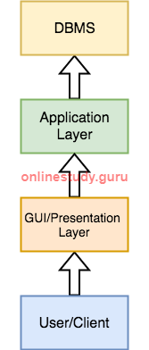
For the end user, the GUI layer is the Database System, and the end user has no idea about the application layer and the DBMS system.
Three-tier architecture typically comprise a presentation tier, a business or data access tier, and a data tier. Three layers in the three tier architecture are as follows:
- Client layer
- Business layer
- Data layer
- Client layer: Represents Web browser, a Java or other application, Applet, WAP phone etc. The client tier makes requests to the Web server who will be serving the request by either returning static content if it is present in the Web server or forwards the request to either Servlet or JSP in the application server for either static or dynamic content.
- Business layer: This layer provides the business services. This tier contains the business logic and the business data. All the business logic like validation of data, calculations, data insertion etc. Are centralized into this tier as opposed to 2-tier systems where the business logic is scattered between the front end and the backend. The benefit of having a centralized business tier is that same business logic can support different types of clients like browser, WAP (Wireless Application Protocol) client, other standalone applications written in Java, C++, C# etc. This acts as an interface between Client layer and Data Access Layer. This layer is also called the intermediary layer helps to make communication faster between client and data layer.
- Data layer: This layer is the external resource such as a database, ERP system, Mainframe system etc. responsible for storing the data. This tier is also known as Data Tier. Data Access Layer contains methods to connect with database or other data source and to perform insert, update, delete, get data from data source based on our input data.
Advantages
- 1. High performance, lightweight persistent objects.
2. Scalability – Each tier can scale horizontally.
3. Performance – Because the Presentation tier can cache requests, network utilization is minimized, and the load is reduced on the Application and Data tiers.
4. Better Re-usability.
5. Improve Data Integrity.
6. Improved Security – Client is not direct access to database.
7. Forced separation of user interface logic and business logic.
8. Business logic sits on small number of centralized machines (may be just one).
9. Easy to maintain, to manage, to scale, loosely coupled etc.
Disadvantages
- 1. Increase Complexity/Effort
Question: -2(b) Describe two alternative for specifying structural constraint on relationship types with an example.
Answer: –

Constraints on Relationship Types
Relationship types usually have certain constraints that limit the possible combinations of entities that may participate in the corresponding relationship set. These constraints are determined from the miniworld situation that the relationships represent. For example, in Figure 7.9, if the company has a rule that each employee must work for exactly one department, then we would like to describe this constraint in the schema. We can distinguish two main types of binary relationship constraints: cardinality ratio and participation.
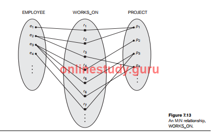
Cardinality for Binary Relationship The cardinality ratio for a binary relationship specifies the maximum number of relationship instances that an entity can participate in. For example, in the WORKS_FOR binary relationship type, DEPARTMENT:EMPLOYEE is of cardinality ratio 1:N, meaning that each department can be related to (that is, employs) any number of employees,9 but an employee can be related to (work for) only one department. This means that for this particular relationship WORKS_FOR, a particular department entity can be related to any number of employees (N indicates there is no maximum number). On the other hand, an employee can be related to a maximum of one department. The possible cardinality ratios for binary relationship types are 1:1, 1:N, N:1, and M:N. An example of a 1:1 binary relationship is MANAGES (Figure 7.12), which relates a department entity to the employee who manages that department. This represents the miniworld constraints that—at any point in time—an employee can manage one department only and a department can have one manager only. The relationship type WORKS_ON (Figure 7.13) is of cardinality ratio M:N, because the mini world rule is that an employee can work on several projects and a project can have several employees. Cardinality ratios for binary relationships are represented on ER diagrams by displaying 1, M, and N on the diamonds. Notice that in this notation, we can either specify no maximum (N) or a maximum of one (1) on participation. An alternative notation allows the designer to specify a specific maximum number on participation, such as 4 or 5.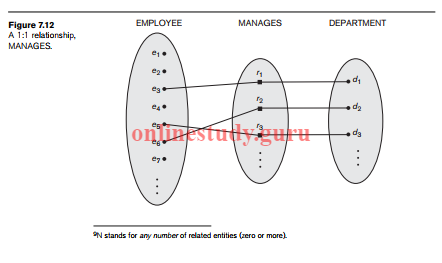
Participation Constraints and Existence Dependencies. The participation constraint specifies whether the existence of an entity depends on its being related to another entity via the relationship type. This constraint specifies the minimum number of relationship instances that each entity can participate in, and is sometimes called the minimum cardinality constraint. There are two types of participation constraints—total and partial—that we illustrate by example. If a company policy states that every employee must work for a department, then an employee entity can exist only if it participates in at least one WORKS_FOR relationship instance (Figure 7.9). Thus, the participation of EMPLOYEE in WORKS_FOR is called total participation, meaning that every entity in the total set of employee entities must be related to a department entity via WORKS_FOR. Total participation is also called existence dependency. In Figure 7.12 we do not expect every employee to manage a department, so the participation of EMPLOYEE in the MANAGES relationship type is partial, meaning that some or part of the set of employee entities are related to some department entity via MANAGES, but not necessarily all. We will refer to the cardinality ratio and participation constraints, taken together, as the structural constraints of a relationship type. In ER diagrams, total participation (or existence dependency) is displayed as a double line connecting the participating entity type to the relationship, whereas partial participation is represented by a single line (see Figure 7.2). Notice that in this notation, we can either specify no minimum (partial participation) or a minimum of one (total participation). The alternative notation (see Section 7.7.4) allows the designer to specify a specific minimum number on participation in the relationship, such as 4 or 5.
- Attributes of Relationship Types
Relationship types can also have attributes, similar to those of entity types. For example, to record the number of hours per week that an employee works on a particular project, we can include an attribute Hours for the WORKS_ON relationship type in Figure 7.13. Another example is to include the date on which a manager started managing a department via an attribute Start_date for the MANAGES relationship type in Figure 7.12. Notice that attributes of 1:1 or 1:N relationship types can be migrated to one of the participating entity types. For example, the Start_date attribute for the MANAGES relationship can be an attribute of either EMPLOYEE or DEPARTMENT, although conceptually it belongs to MANAGES. This is because MANAGES is a 1:1 relationship, so every department or employee entity participates in at most one relationship instance. Hence, the value of the Start_date attribute can be determined separately, either by the participating department entity or by the participating employee (manager) entity. For a 1:N relationship type, a relationship attribute can be migrated only to the entity type on the N-side of the relationship. For example, in Figure 7.9, if the WORKS_FOR relationship also has an attribute Start_date that indicates when an employee started working for a department, this attribute can be included as an attribute of EMPLOYEE. This is because each employee works for only one department, and hence participates in at most one relationship instance in WORKS_FOR. In both 1:1 and 1:N relationship types, the decision where to place a relationship attribute—as a relationship type attribute or as an attribute of a participating entity type—is determined subjectively by the schema designer. For M:N relationship types, some attributes may be determined by the combination of participating entities in a relationship instance, not by any single entity. Such attributes must be specified as relationship attributes. An example is the Hours attribute of the M:N relationship WORKS_ON (Figure 7.13); the number of hours per week an employee currently works on a project is determined by an employeeproject combination and not separately by either entity.
Question: – 3(a) Discuss different types of user-friendly interfaces and database utility and list the common function that the utility perform.
Answer: – User-friendly interfaces
User-friendly interfaces provided by a DBMS may include the following: Menu-Based Interfaces for Web Clients or Browsing. These interfaces present the user with lists of options (called menus) that lead the user through the formulation of a request. Menus do away with the need to memorize the specific commands and syntax of a query language; rather, the query is composed step-bystep by picking options from a menu that is displayed by the system. Pull-down menus are a very popular technique in Web-based user interfaces. They are also often used in browsing interfaces, which allow a user to look through the contents of a database in an exploratory and unstructured manner. Forms-Based Interfaces. A forms-based interface displays a form to each user. Users can fill out all of the form entries to insert new data, or they can fill out only certain entries, in which case the DBMS will retrieve matching data for the remaining entries. Forms are usually designed and programmed for naive users as interfaces to canned transactions. Many DBMSs have forms specification languages, which are special languages that help programmers specify such forms. SQL*Forms is a form-based language that specifies queries using a form designed in conjunction with the relational database schema. Oracle Forms is a component of the Oracle product suite that provides an extensive set of features to design and build applications using forms. Some systems have utilities that define a form by letting the end user interactively construct a sample form on the screen. Graphical User Interfaces. A GUI typically displays a schema to the user in diagrammatic form. The user then can specify a query by manipulating the diagram. In many cases, GUIs utilize both menus and forms. Most GUIs use a pointing device, such as a mouse, to select certain parts of the displayed schema diagram.
Database System Utilities:- In addition to possessing the software modules just described, most DBMSs have database utilities that help the DBA manage the database system. Common utilities have the following types of functions: ■ Loading. A loading utility is used to load existing data files—such as text files or sequential files—into the database. Usually, the current (source) for- mat of the data file and the desired (target) database file structure are specified to the utility, which then automatically reformats the data and stores it in the database. With the proliferation of DBMSs, transferring data from one DBMS to another is becoming common in many organizations. Some vendors are offering products that generate the appropriate loading programs, given the existing source and target database storage descriptions (internal schemas). Such tools are also called conversion tools. For the hierarchical DBMS called IMS (IBM) and for many network DBMSs including IDMS (Computer Associates), SUPRA (Cincom), and IMAGE (HP), the vendors or third-party companies are making a variety of conversion tools available (e.g., Cincom’s SUPRA Server SQL) to transform data into the relational model. ■ Backup. A backup utility creates a backup copy of the database, usually by dumping the entire database onto tape or other mass storage medium. The backup copy can be used to restore the database in case of catastrophic disk failure. Incremental backups are also often used, where only changes since the previous backup are recorded. Incremental backup is more complex, but saves storage space. ■ Database storage reorganization.This utility can be used to reorganize a set of database files into different file organizations, and create new access paths to improve performance. ■ Performance monitoring. Such a utility monitors database usage and provides statistics to the DBA. The DBA uses the statistics in making decisions such as whether or not to reorganize files or whether to add or drop indexes to improve performance. Other utilities may be available for sorting files, handling data compression, monitoring access by users, interfacing with the network, and performing other functions.
Question: – 3(b) Why E-R model is considered as high level conceptual model? Discuss the role of high level model in database design process.
Answer: –
The three levels of data modeling, conceptual data model, logical data model, and physical data model, were discussed in prior sections. Here we compare these three types of data models. The table below compares the different features:
| Feature | Conceptual | Logical | Physical |
| Entity Names | ✓ | ✓ | |
| Entity Relationships | ✓ | ✓ | |
| Attributes | ✓ | ||
| Primary Keys | ✓ | ✓ | |
| Foreign Keys | ✓ | ✓ | |
| Table Names | ✓ | ||
| Column Names | ✓ | ||
| Column Data Types | ✓ |
Conceptual Data Model
A conceptual data model identifies the highest-level relationships between the different entities. Features of conceptual data model include:
- Includes the important entities and the relationships among them.
- No attribute is specified.
- No primary key is specified.
The figure below is an example of a conceptual data model.
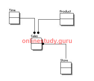
From the figure above, we can see that the only information shown via the conceptual data model is the entities that describe the data and the relationships between those entities. No other information is shown through the conceptual data model.
Logical Data Model
A logical data model describes the data in as much detail as possible, without regard to how they will be physical implemented in the database. Features of a logical data model include:
- Includes all entities and relationships among them.
- All attributes for each entity are specified.
- The primary key for each entity is specified.
- Foreign keys (keys identifying the relationship between different entities) are specified.
- Normalization occurs at this level.
The steps for designing the logical data model are as follows:
- Specify primary keys for all entities.
- Find the relationships between different entities.
- Find all attributes for each entity.
- Resolve many-to-many relationships.
The figure below is an example of a logical data model.

Comparing the logical data model shown above with the conceptual data model diagram, we see the main differences between the two:
- In a logical data model, primary keys are present, whereas in a conceptual data model, no primary key is present.
- In a logical data model, all attributes are specified within an entity. No attributes are specified in a conceptual data model.
- Relationships between entities are specified using primary keys and foreign keys in a logical data model. In a conceptual data model, the relationships are simply stated, not specified, so we simply know that two entities are related, but we do not specify what attributes are used for this relationship.
Physical Data Model
Physical data model represents how the model will be built in the database. A physical database model shows all table structures, including column name, column data type, column constraints, primary key, foreign key, and relationships between tables. Features of a physical data model include:
- Specification all tables and columns.
- Foreign keys are used to identify relationships between tables.
- Denormalization may occur based on user requirements.
- Physical considerations may cause the physical data model to be quite different from the logical data model.
- Physical data model will be different for different RDBMS. For example, data type for a column may be different between MySQL and SQL Server.
The steps for physical data model design are as follows:
- Convert entities into tables.
- Convert relationships into foreign keys.
- Convert attributes into columns.
- Modify the physical data model based on physical constraints / requirements.
The figure below is an example of a physical data model.
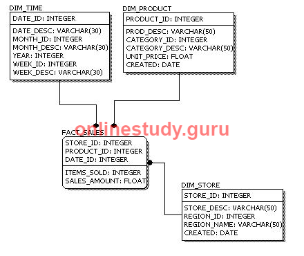
Comparing the physical data model shown above with the logical data model diagram, we see the main differences between the two:
- Entity names are now table names.
- Attributes are now column names.
- Data type for each column is specified. Data types can be different depending on the actual database being used.
This article is contributed by Tarun Jangra. Please write comments if you find anything incorrect, or you want to share more information about the topic discussed above.


your article I understand completely sir.
Thanks for your Complement.
vb ka paper exam se kitna phle aa jayega sir
Tomorrow 5:00 pm
But solution are available something after 6:00 pm. so, you can check question paper only at 5:00 pm and solution after 6:00 pm.