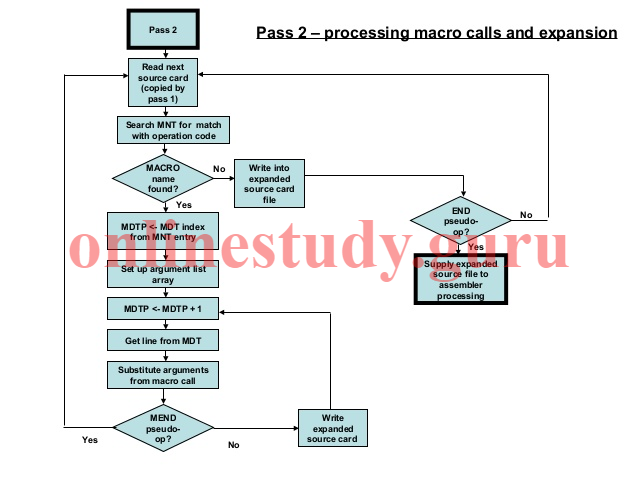
Question: – 2(a) Explain the problems faced by a one-pass assembler. Draw and explain the detailed flowchart for pass-2 of a two pass assembler.
Answer:- Single pass assemblerSingle Pass Assembler . A single pass assembler scans the program only once and creates the equivalent binary program. The assembler substitute all of the symbolic instruction with machine code in one pass.. Advantages Every source statement needs to be processed once. . Disadvantages We cannot use any forward reference in our program.. Forward Reference Forward reference means; reference to an instruction which has not yet been encountered by the assembler. In order to handle forward reference, the program needs to be scanned twice. In other words a two pass assembler is needed.
- Similarly, A one-pass assembler requires 1 scan of the source program to generate machine code.
- Moreover, The process of forwarding references talked using a process called back patching. The operand field of an instruction containing forward references left blank initially.
- Also, A table of instruction containing forward references maintained separately.
Disadvantage:-
The disadvantage of a single pass assembler over a 2 pass assembler, where they both generate an executable (No linker).
So a single pass assembler, the biggest problems is forward references. The classic problem of if you jump to a forward label, it won’t know automatically if you need a near, or a far jump. So you either have to state it explicitly, or the assembler may have to just make everything far.
Any forwarding label reference will cause problems. Suppose you want to compile in an array of chars, and you want to calculate it’s size. You can only do this calculation AFTER the definition. You can’t place it before in a single pass assembler, because it won’t know those addresses until the compiler has already gone past them.
The other big disadvantage, is a single pass assemblers traditionally don’t really generate a symbol table, or object code. So you can’t “link” it with anything else. There is no object file generated so that you can link it with other languages, or other assembly modules.

Two-pass assembler: Assemblers typically make two or more passes through a source program in order to resolve forward references in a program. A forward reference is defined as a type of instruction in the code segment that is referencing the label of an instruction, but the assembler has not yet encountered the definition of that instruction.
Pass 1: Assembler reads the entire source program and constructs a symbol table of names and labels used in the program, that is, name of data fields and programs labels and their relative location (offset) within the segment.
Pass 1 determines the amount of code to be generated for each instruction.
Pass 2: The assembler uses the symbol table that it constructed in Pass 1. Now it knows the length and relative of each data field and instruction, it can complete the object code for each instruction. It produces .OBJ (Object file), .LST (list file) and cross reference (.CRF) files.
- Two pass translations consist of pass I and pass II.
- Generally, LC processing performed in the first pass and symbols defined in the program entered into the symbol table, hence first pass performs analysis of the source program.
- So, two pass translation of assembly lang. the program can handle forward reference easily.
- The second pass synthesizes the target form using the address information found in the symbol table.
- Moreover, The first pass constructs an intermediate representation of the source program and that will be used by the second pass.
- IR consists of two main components: data structure + IC (intermediate code)
Question: – 2(b) what are Different loading Schemes? Explain absolute loader scheme with its advantages and disadvantages.
Answer:- Loading Schemes
1. Absolute loader:-The task of an absolute loader is virtually trivial.The loader simply accepts machine language code and places it into main memory specified by the assembler.
- An absolute loader loads a binary program in memory for execution.
- The binary program is stored in a file contains the following:
- A Header record showing the load origin, length and load time execution start address of the program.
- A sequence of binary image records containing the program’s code. Each binary image record contains a part of the program’s code in the form of a sequence of bytes, the load address of the first byte of this code and a count of the number of bytes of code.
- The absolute loader notes the load origin and the length of the program mentioned in the
header record. - It then enters a loop that reads a binary image record and moves the code contained in it
to the memory area starting at the address mentioned in the binary image record. - At the end, it transfers control to the execution start address of the program.
Advantages of the absolute loading scheme: Absolute Loaders
Simple to implement and efficient in execution.
Moreover, Saves the memory (core) because the size of the loader is smaller than that of the assembler.
Allows use of multi-source programs written in different languages. In such cases, the given language assembler converts the source program into the language. And a common object file is then prepared by address resolution.
The loader is simpler and just obeys the instruction regarding where to place the object code in the main memory.
Disadvantages of the absolute loading scheme: Absolute Loaders
o The programmer must know and clearly specify to the translator (the assembler) the address in the memory for inner-linking and loading of the programs. Care should take so that the addresses do not overlap.
o For programs with multiple subroutines, the programmer must remember the absolute address of each subroutine and use it explicitly in other subroutines to perform linking.
o If the subroutine is modified, the program has to assemble again from first to last.
2. Relocating loader:- The task of relocating loader is to avoid reassembling of of all subroutines when a subroutine is changed and to perform tasks of allocation and linking for programmer.
3. Dynamic Loading:- In order to overlay structure to work it is necessary for the module loader to load the various procedures as they are needed.There are many binders capable of processing and allocating overlay structure.the portion of the laoder that actually intercepts calls and loads necessary procedure is called overlay supervisor of simplly flipper.this overall scheme is called dynamic loading or load on call.
4. Dynamic linking:- This is mechanism by which loading and linking of external references are postponed until execution time.This was made to sort out disadvantage of previous loading schemes like subroutine is referenced and never executed
5. General Loader Schemes:-
- The general loading scheme improves the compile/assemble-and-go scheme by allowing
different source programs (or modules of the same program) to be translated separately
into their respective object programs. - Moreover, The object code (modules) stored in the secondary storage area; and then, they are
loaded. - Similarly, The loader usually combines the object codes and executes them by loading them into the
memory, including space where the assembler had been in the assemble-and-go
scheme. - Rather than the entire assembler sitting in the memory, a small utility component called
loader does the job. - Note that the loader program is comparatively much smaller than the assembler, hence
making more space available to the user for their programs.Advantages of the general loading scheme: Different Loading Schemes:-
Saves memory and makes it available for the user program as loaders are smaller in size than assemblers. The loader replaces the assembler.
Similarly, Reassembly of the program no more needed for later execution of the program.
The object file/deck available and can load and executed directly at the desired location.This scheme allows the use of subroutines in several different languages because the object files processed by the loader utility will all be in machine language.
Disadvantages of the general loading scheme
Moreover, The loader more complicated and needs to manage multiple object files.
Secondary storage required to store object files, and they cannot directly place into the memory by assemblers.
Question: -3(a) What are the basics function of loaders? Differentiate linking, relative and bootstrap loader.
Answer:- Definitions of Loader:
A loader is a major component of an operating system that ensures all necessary programs and libraries are loaded, which is essential during the startup phase of running a program. It places the libraries and programs into the main memory in order to prepare them for execution. Loading involves reading the contents of the executable file that contains the instructions of the program and then doing other preparatory tasks that are required in order to prepare the executable for running, all of which takes anywhere from a few seconds to minutes depending on the size of the program that needs to run.
The loader is a component of an operating system that carries out the task of preparing a program or application for execution by the OS. It does this by reading the contents of the executable file and then storing these instructions into the RAM, as well as any library elements that are required to be in memory for the program to execute. This is the reason a splash screen appears right before most programs start, often showing what is happening in the background, which is what the loader is currently loading into the memory. When all of that is done, the program is ready to execute. For small programs, this process is almost instantaneous, but for large and complex applications with large libraries required for execution, such as games as well as 3D and CAD software, this could take longer. The loading speed is also dependent on the speed of the CPU and RAM.
Not all code and libraries are loaded at program startup, only the ones required for actually running the program. Other libraries are loaded as the program runs, or only as required. This is especially true for applications such as games that only need assets loaded for the current level or location that the player is in.
Though loaders in different operating systems might have their own nuances and specialized functions native to that particular operating system, they still serve basically the same function. The following are the responsibilities of a loader:
- Validate the program for memory requirements, permissions, etc.
- Copy necessary files, such as the program image or required libraries, from the disk into the memory
- Copy required command-line arguments into the stack
- Link the starting point of the program and link any other required library
- Initialize the registers
- Jump to the program starting point in memory
The basic functions of loaders
1. Loading – brings the object program into memory for execution
- Bootstrapping
- Actions taken when a computer is first powered on
- The hardware logic reads a program from address 0 of ROM (Read Only Memory)
- ROM is installed by the manufacturer
- ROM contains bootstrapping program and some other routines that controls hardware (e.g. BIOS)
- Bootstrapping is a loader
- Loads OS from disk into memory and makes it run
- The location of OS on disk (or floppy) usually starts at the first sector
- Starting address in memory is usually fixed to 0
- no need of relocation
- This kind of loader is simple
- no relocation
- no linking
- called “absolute loader”
- Relocation– modifies the object program so that it can be loaded at an address different from the location originally specified
- Assembler review
- Assembler generates an object code assuming that the program starts at memory address 0
- Loader decides the starting address of a program
- Assembler generates modification record
- Limits of modification record
- Record format
- (address, length)
- It can be huge when direct addressing is frequently used
- If instruction format is fixed for absolute addressing, the length part can be removed
- Instead of address field, bit-vector can be used
- …. means instruction 1 2 4 5. .. need to be modified
- Hardware support for relocation
- Base register
- assembler and loader do not need to worry about relocation
- Base register
- Record format
- Linking– combines two or more separate object programs and also supplies the information needed to reference them.
- Background
- A large problem is better broken into several small pieces
- Each piece is better implemented independently
- assembled (compiled) independently
- There are many data structures shared among those pieces
- variables and procedures
- Some programs are used by many different programs
- print(), file operations, exp(), sin(), …
- these are usually provided as library functions
- Requirements for linking
- Each module defines
- which symbols are used by other modules
- symbols undefined in a module are assumed to be defined in other modules
- if these symbols are declared explicitly, it helps linker to resolve
- Principles
- Assembler evaluates as much as possible
- expressions
- If some cannot be resolved,
- provide the modification records
Question: -3(b) State the basics tasks a macro instruction processor performs. Explain how the nested macro calls are executed with an example.
Answer:- Basic tasks : Macro Instruction
A macro instruction is a group of programming instructions that have been compressed into a simpler form and appear as a single instruction. When used, a macro expands from its compressed form into its actual instruction details. Both the name of the macro definition and other variable parameter attributes are included within the macro statement.
onlinestudy.guru –> explains Macro Instruction
Macro instructions were first used in the assembler language rather than a higher-level programming language. The way a macro expands to a set of instructions depends on the macro definition, which converts the macro into its detailed instructional form.
Macros save developers much time and effort, especially when dealing with a certain sequence of commands that is repeated more than once within the program body. Macros also save space and spare the programmer time spent on a long code block that may pertain to performing a single function.
The concept of macros is used within some precompilers, while higher-level languages focus on simplifying program and function writing, which makes the macro instruction a common element among most high-level programming languages. Macro instructions are generated together with the rest of the program by the assembler.
Basic macro processor functions/task
Two new assembler directives are used in macro
definition
MACRO: identify the beginning of a macro definition
MEND: identify the end of a macro definition
Prototype for the macro
Each parameter begins with ‘&’
name MACRO parameters
:
body
:
MEND
Body: the statements that will be generated as the expansion of the
macro.
Nested Macro Calls:
Macro bodies may also contain macro calls, and so may the bodies of those called macros, and so forth.
If a macro call is seen throughout the expansion of a macro, the assembler starts immediately with the expansion of the called macro. For this, its its expanded body lines are simply inserted into the expanded macro body of the calling macro, until the called macro is completely expanded. Then the expansion of the calling macro is continued with the body line following the nested macro call.
Example 1:
        INSIDE MACRO
        SUBB A,R3
        ENDM

        OUTSIDE MACRO
        MOV A,#42
        INSIDE
        MOV R7,A
        ENDM
In the body of the macro OUTSIDE, the macro ISIDE is called. If OUTSIDE is called (and the list mode is set to $GENONLY), one gets something like the following expansion:
        Line  I  Addr  Code            Source

          15+ 1  0000  74 2A           MOV A,#42
          17+ 2  0002  9B              SUBB A,R3
          18+ 1  0003  FF              MOV R7,A
Since macro calls can be nested to any depth (while there is free memory), the macro expansion level is shown in the I-column of the list file. Since macro and include file levels can be nested in arbitrary sequence and depth, the nesting level is counted through all macro and include file levels regardless. For better distinction, the character following the global line number is ‘:’ for include file levels, and ‘+’ for macro levels.
If macros are calling themselves, one speaks of recursive macro calls. In this case, there must be some stop criterion, to prevent the macro of calling itself over and over until the assembler is running out of memory! Here again, conditional assembly is the solution:
Example 2:
The macro COUNTDOWN is to define 16-bit constants from 1 thru n in descending order in ROM. n can be passed to the macro as a parameter:
        COUNTDOWN MACRO DEPTH
        IF DEPTH GT 0
        DW DEPTH
        COUNTDOWN %DEPTH-1
        ENDIF
        ENDM
If COUNTDOWN is called like this,
COUNTDOWN 7
something like the following macro expansion results (in list mode $GENONLY/$CONDONLY):
        Line  I  Addr  Code            Source

          16+ 1  0000  00 07           DW 7
          19+ 2  0002  00 06           DW 6
          22+ 3  0004  00 05           DW 5
          25+ 4  0006  00 04           DW 4
          28+ 5  0008  00 03           DW 3
          31+ 6  000A  00 02           DW 2
          34+ 7  000C  00 01           DW 1
After the Dark Ages, when the dust was settling and the sun broke through the gloom, computer science discovered the method of recursive programming. There was no doubt that this was the Solution!
And the computer scientists started to explain this to the students. But it seemed that the students didn’t get it. They always complained that recursive calculation of n! is a silly example indeed.
All the scientists felt stronly that there was still something missing. After 10 more years of hard research work, they also found the Problem.
This article is contributed by Tarun Jangra. Please write comments if you find anything incorrect, or you want to share more information about the topic discussed above.